Simple winning streak simulation
(c) Jussi Palomäki, 2023
Below is a simple simulation for winning streak lengths when the outcome is either a “win” with 85% probability or a “loss” with 15% probability.
I’m using a streak length of 44 as a “length of interest”. If 50 000 games are played given these probabilities, then the likelihood of not having a winning streak of at least 44 games at least once, is 0.6% (0.006). Over a period of 50 000 games given the above probabilities for wins and losses, one should on average expect to have 4.961 winning streaks (SD = 2.232143) that are at least 44 games long.
I also visualize the distribution of the longest winning streaks for each 1000 simulated set of 50 thousand games. As can be seen in the figure (histogram), even winning streaks of 80+ games are certainly not unheard of, given these parameters.
Simulations
library(tidyverse)

#Loss = 0, Win = 1
result <- c(0, 1)

#Probability for Loss = 15 %, probability for Win = 85 % (roughly approximating an elo-rating difference of 300)
probability <- c(0.15, 0.85)

#Streak length of interest
streak <- 44

#Number of games played
games <- 50000

#How many times we iterate over the simulation
replicates <- 1000

#Simulate sample of 50000 games such that in each game, we win 85% of the time and lose 15% of the time
#Result: list of 0s and 1s for each game (display first 30)
set.seed(1)
head(sample(result, games, replace=TRUE, prob = probability), 30)
## [1] 1 1 1 0 1 0 0 1 1 1 1 1 1 1 1 1 1 0 1 1 0 1 1 1 1 1 1 1 0 1#For these games, calculate the length of each win streak.
#Result: list of winning streak lengths across all 50000 games (display first 30)
set.seed(1)
run_length_all <- rle(sample(result, games, replace=TRUE, prob = probability))
run_length_wins <- run_length_all$lengths[run_length_all$values==1]
run_length_losses <- run_length_all$lengths[run_length_all$values==0] #to be used later (not yet analysed)
head(run_length_wins, 30)## [1] 3 1 10 2 7 22 8 8 5 2 13 9 4 1 9 13 3 10 11 2 7 2 3 2 1
## [26] 3 4 16 2 3#Calculate the number of winning streaks longer than 44
sum(run_length_wins > streak)## [1] 4#Calculate the number of winning streaks longer than 44 1000 times, obtain mean and standard deviation
set.seed(1)
run_length_wins_repl <- replicate(replicates, with(rle(sample(result, games, replace=TRUE, prob = probability)), sum(lengths[values==1] > streak)))
head(run_length_wins_repl, 30)## [1] 4 7 5 3 4 4 2 6 8 8 6 6 5 6 3 5 4 6 4 3 7 4 5 5 5 4 4 2 4 9mean(run_length_wins_repl)## [1] 4.961sd(run_length_wins_repl)## [1] 2.232143#Calculate the number of times there were 0 winning streaks of at least 44 games, express it as a probability
set.seed(1)
sum(run_length_wins_repl == 0) / replicates## [1] 0.006Histogram
#Histogram showing the distribution of the maximum streak lengths across all simulations
set.seed(1)
chess_data <- tibble(x = replicate(replicates, with(rle(sample(result, games, replace=TRUE, prob = probability)), max(lengths[values==1]))))

chess_data %>% ggplot(aes(x)) +
  geom_bar(aes(y = (..count..)/sum(..count..)), color = "black", fill = "lightblue") +
  #geom_histogram(aes(y=..density..), color = "black", fill = "lightblue") +
  #geom_density() +
  scale_y_continuous(labels = scales::label_percent(accuracy = 1L)) +
  labs(y = "Proportion", x = "Maximum winning streak length (number of games)",
       title = "50k games played simulated 1000 times, 300 elo difference (15% / 85%)") +
  theme_bw()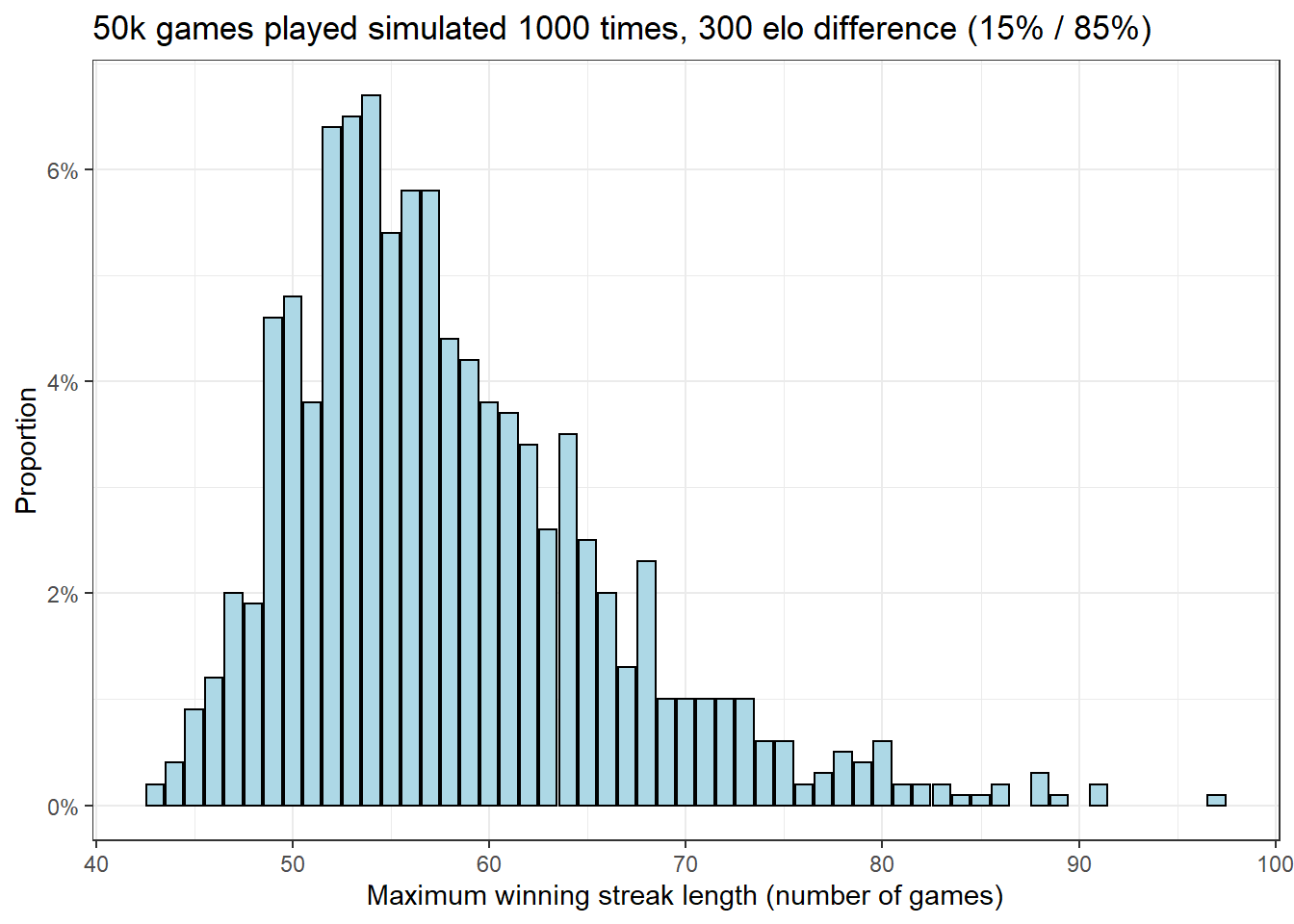
Histogram comparisons (hypothetical cheaters vs. legit players)
#Histogram showing the distribution of the maximum streak lengths across all simulations, separetely for hypothetical cheaters (with 80% win probability) and legit players (with 70% win probability)
set.seed(1)
probability_cheaters <- c(0.2, 0.8)
probability_legit <- c(0.30, 0.70)

chess_data_cheaters <- tibble(x = replicate(replicates, with(rle(sample(result, games, replace=TRUE, prob = probability_cheaters)), max(lengths[values==1]))), group = "Cheaters (80% win)")
chess_data_legit <- tibble(x = replicate(replicates, with(rle(sample(result, games, replace=TRUE, prob = probability_legit)), max(lengths[values==1]))),
                           group = "Legit players (70% win)")

chess_data_all <- rbind(chess_data_cheaters, chess_data_legit)


chess_data_all %>% ggplot(aes(x, fill = group, color = group)) +
  #geom_density(aes(color = group, fill = group), alpha=.5) +
  geom_bar(aes(y = (..count..)/sum(..count..)), alpha = .25, position = "identity") +
  #geom_histogram(aes(y=..density..), color = "black", fill = "lightblue") +
  scale_y_continuous(labels = scales::label_percent(accuracy = 1L)) +
  labs(y = "Proportion", x = "Maximum winning streak length (number of games)",
       title = "50k games played simulated 1000 times") +
  theme_bw(base_size=13) +
  theme(legend.position = c(0.7,0.5)) +
  # scale_fill_manual(values = c("salmon", "blue")) +
  # scale_color_manual(values = c("salmon", "blue")) +
  labs(color = NULL, fill = NULL)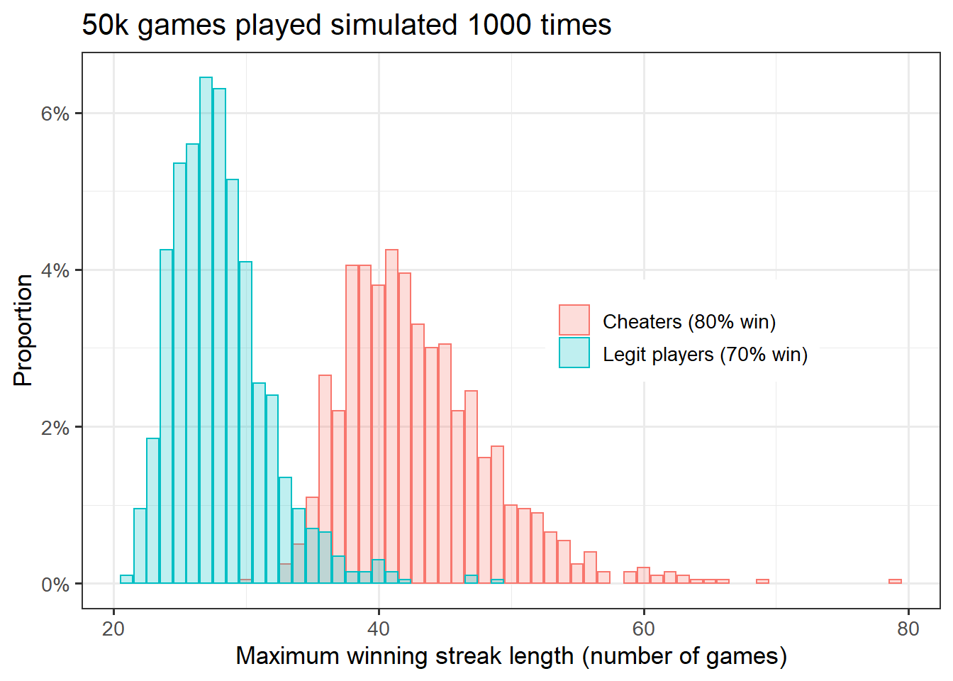
#wilcox.test(chess_data_all$x~chess_data_all$group)